
This post serves as a practical approach towards a vectorized implementation of the Expectation Maximization (EM) algorithm mainly for MATLAB or OCTAVE applications. EM is a really powerful and elegant method for finding maximum likelihood solutions in cases where the hypothesis involves a gaussian mixture model and latent variables.
Introduction
EM is connected with the maximization of the (log-)likelihood function of a general form that includes a gaussian mixture of K gaussians as follows:

|
(1) |
where,

Apparently the multi-variate gaussian (normal) distribution follows the generalized pdf definition:
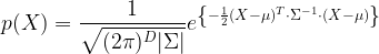
|
(2) |
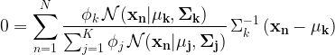
EM is an iterative optimization method which in essence maximizes the likelihood. Maximization of (1) in respect to the means of the gaussians results:
|
(3) |
which includes no other than what is called the responsibility that the gaussian 


|
(4) |
Solving (3) for the means of each gaussian:
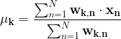
|
(5) |
Solving (3) for the covariances of each gaussian:
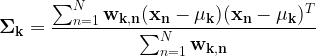
|
(6) |
Solving (3) for the mixing coefficient of each gaussian, requires the application of Lagrange multipliers, which eventually results:
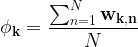
|
(7) |
which says that the mixing coefficient for the gaussian
Putting it all together, the EM algorithm is as follows:
- Initialization: Initialization of means, covariances and mixing coefficients (and estimation of the log-likelihood (1).
- E-step (Expectation): Estimation of the responsibilities (4).
- M-step (Maximization): Re-estimation of the means (5), covariances (6) and mixing coefficients (7).
- Evaluation: Evaluation of the log-likelihood (1) and check for convergence of either the log-likelihood or the other parameters (basically the means).
* A note on initialisation: As in many iterative methods, initial conditions are extremely important. It has been proposed that a quick k-means on the data could result in a good initial estimate of the clusters in the dataset (means and covariances).
So how is this transformed into a vectorized form for efficient MATLAB/OCTAVE implementation?
Suppose we start with 


At first lets say we initialize by a k-means:
[ labels, centroids ] = kmeans( X, classes);
for k = 1:classes
	m{k} = centroids(k,:)';
	s{k} = cov( X( find(labels==k), : ) );
end
% initial prior probabilities for each cluster (all equal)
phi = (ones(classes,1) * (1 / classes));
Then comes the E-step of the algorithm as follows:
g = zeros( samples, classes);
for k=1:classes
	% compute the probability that the gaussian i produces input vector X(j,:)
	% g is NxD
	% typical array multiplication
	% g(:,k) = exp(-0.5 * diag((X-m{k}') * inv(s{k}) * (X-m{k}')')) / sqrt((2*pi)^dims * det(s{k}));
	% faster implementation
	g(:,k) = exp(-0.5 * sum((X-m{k}') * inv(s{k}) .* (X-m{k}'),2)) / sqrt((2*pi)^dims * det(s{k}));
end
% compute the responsibility of each class producing each input data vector X belongs to each class
% w is NxD
w = g.*phi';
w = w ./ sum(w,2);
Next comes the more complicated M-step as follows:
% store the current means
currM = m;
% calculate the new prior probabilities based on the means
phi = mean(w,1)';
% Calculate the new means for each of the classes/distributions
mm = (w'*X)'./sum(w,1);
for k=1:classes
	% update the mean of the class/distribution
	m{k} = mm(:,k);
	% update the covariance matrix of the class/distribution
	Xm = X - m{k}';
	XmT = (w(:,k).*Xm)';
	s{k} = (XmT*Xm) / sum(w);
end
Apparently the above E-step and M-step are within a loop, for example:
for iter = 1:iterations
	% E-step
	% M- step
	% check for convergence
end
Checking for convergence could be based on the log-likelihood update:
% could be an estimate of the motion of the means
error = sum(diag(pdist2(cell2mat(m)',cell2mat(currM)','euclidean')));

% Bishop suggests evaluating the log likelihood and checking conversion on the likelihood or the parameters
llg = sum( log( sum(g.*phi',2)));
error = abs( llg - sum( log( sum(w,2))));
Let’s take a look at an example
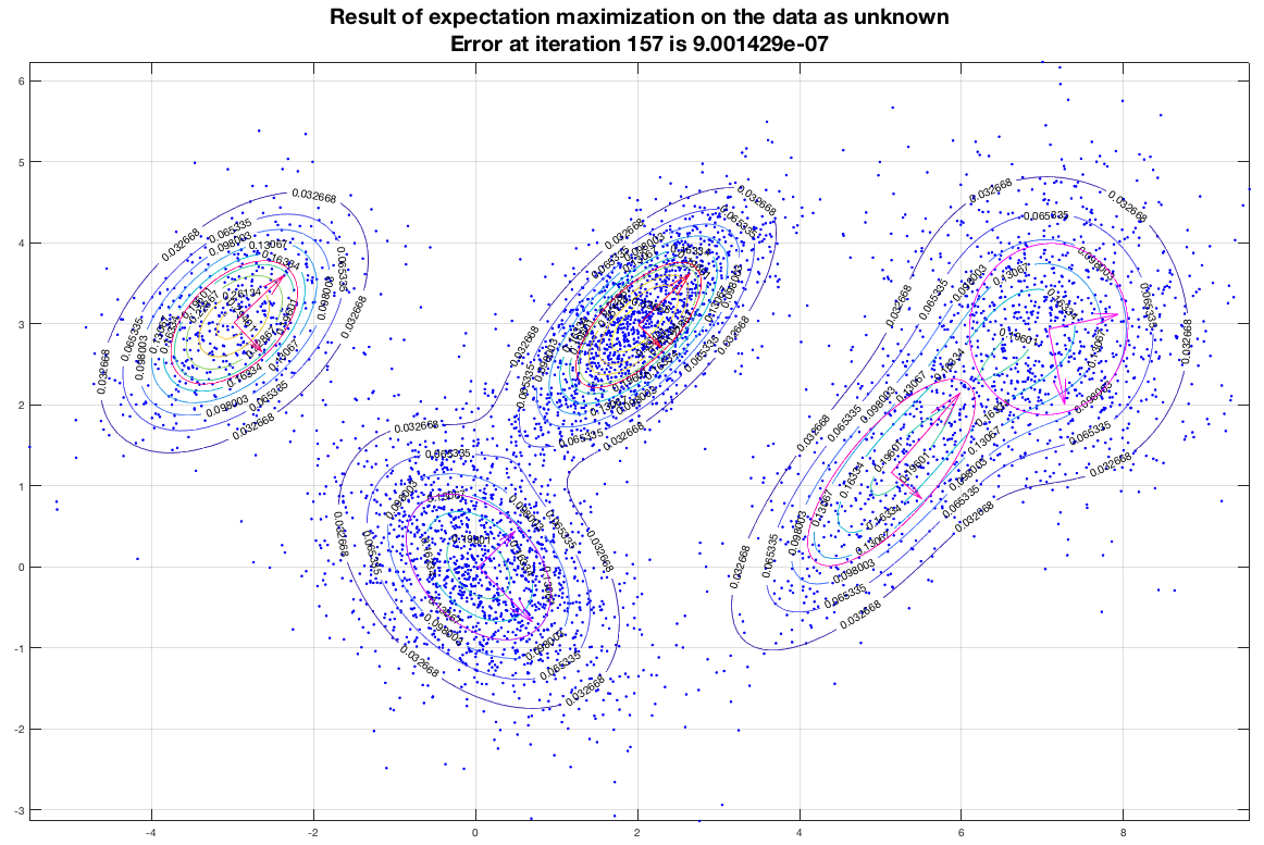
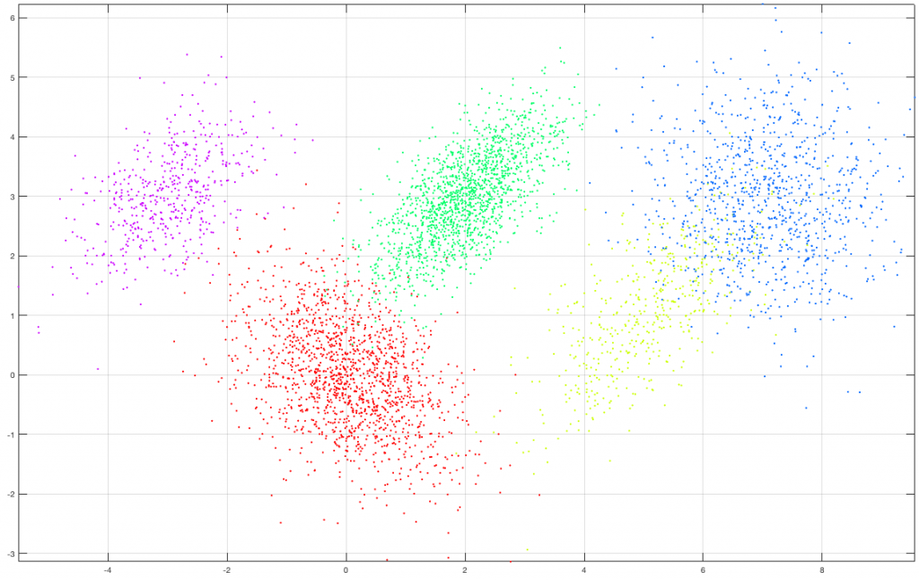
Suppose we create a set of 5000 2D observations drawn from a mixture of five (5) gaussians of various means and covariances with a specific set of mixing coefficients as shown in the following figure. Each class (gaussian) is denoted by a different color in the graph.
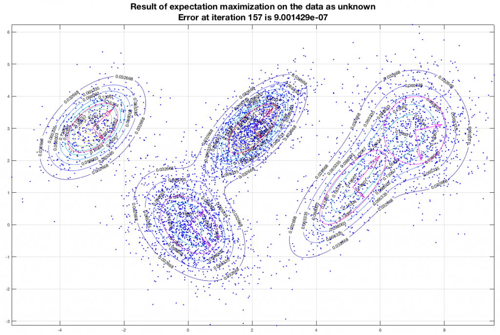
Running the EM algorithm on these data and imposing that we want to end up with five (5) gaussians we get a result that is depicted in the following figure. In this figure, the contours represent equiprobable curves around the recognized gaussian distributions, the vectors in the center of each gaussian is a representation of the corresponding (square roots of the) eigenvectors (of the covariance matrix). The algorithm has converged after 157 iterations as shown, and the final estimate of the means of the gaussians moved only about 9×10⁻⁷ from their semi-final estimate.
Bibliography
1. Bishop, C. (2007). Pattern Recognition and Machine Learning (Information Science and Statistics), 1st edn. 2006. corr. 2nd printing edn. Springer, New York.
2. Theodoridis, S., Pikrakis, A., Koutroumbas, K., & Cavouras, D. (2010). Introduction to pattern recognition: a matlab approach. Academic Press.
3. Zafeiriou, S. (2015). Tutorial on Expectation Maximization (Example). Online @ https://ibug.doc.ic.ac.uk/media/uploads/documents/expectation_maximization-1.pdf.
4. McCormick, C. (2014-updated 2017).Gaussian Mixture Models Tutorial and MATLAB Code. Online @ http://mccormickml.com/2014/08/04/gaussian-mixture-models-tutorial-and-matlab-code/.
