
A straightforward approach to do geometric image transformations using MATLAB is to take advantage of the imtransform function available.
First the image is supposed to be within a ‘unity’ rectangle and initial transformation conditions are defined accordingly:
udata = [0 1];
vdata = [0 1];
fill_color = 128;
org_rect = [0 0;1 0;1 1;0 1];
The fill_color variable represents just the color to be used for filling the parts of the canvas that will not be covered by the transformed image. Then a projective transformation can be applied to project the original to the new rectangle representing the image canvas as follows:
tform = maketform('projective', org_rect, new_rect);
[out_im,xdata,ydata] = imtransform( in_im, tform, 'bicubic', 'udata', udata, 'vdata', vdata, 'size', size(in_im), 'fill', fill_color);
Notice that the transformation is bicubic and returns both the out image (out_im) and the new coordinate system represented by xdata and ydata.
If only the output image is kept then it will be of the same size as the input image in the original coordinate system (so it will be somehow stretched). In order to display the images properly the following command may be used:
imshow(out_im,'XData',xdata,'YData',ydata);
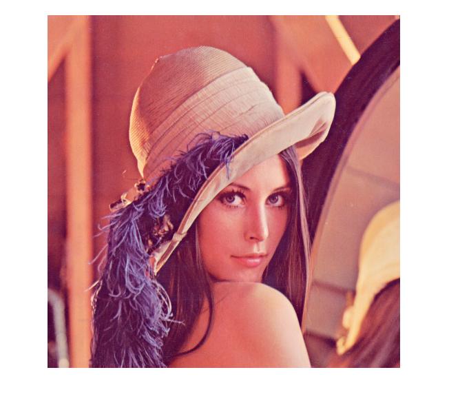
Here is an example. Let’s considered the case of Lena shown below:
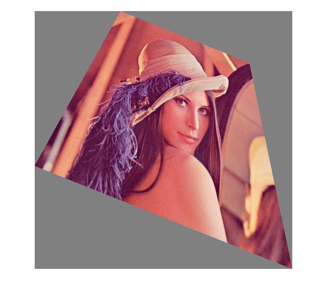
After applying the transformation we may display using the correct coordinates as shown below:
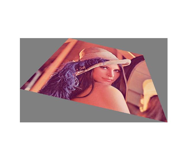
If the output image is displayed without any reference to the new coordinate system the image will be stretched as shown below:

The output rectangle used in this example was: [-1 -2;2 -1;3 3;-3 1]
