
Machine learning is a research domain that is becoming the holy grail of data science towards the modelling and solution of science and engineering problems. I have already witnessed researchers proposing solutions to problems out of their area of expertise using machine learning methods, basing their approach on the success of modern machine learning algorithm on any kinds of data. Apparently this is not a good choice and I have also witnessed failures, since those modern methods in many cases rely on an intuition on the data at hand. Nevertheless, the particular field of deep learning with artificial neural networks has already successfully proposed significant solutions to highly complex problems in a diverse range of domains and applications.
Usually learning about these methods starts off with the general categorisation of problems into regression and classification, the first tackling the issue of learning a model (usually also called a hypothesis) that fits the data and the second focusing on learning a model that categorises the data into classes. The simpler case in classification is what is called binary (or binomial) classification, in which the task is to identify and assign data into two classes. A more complex case is the case of multi-class classification, in which data are to be assigned to more than two classes.
Regression, and particularly linear regression is where everyone starts off. Linear regression focuses on learning a line that fits the data. The way it works is based on an iterative minimisation of a kind of an error of the predictions of the current model to the actual solution (which is known during training). Gradient descent is usually the very first optimisation algorithm presented that can be used to optimise a cost function, which is arbitrarily defined to measure the cost of using specific parameters for a hypothesis (model) in relation to the correct choice. Gradient descent intuitively tries to find the lower limits of the cost function (thus the optimum solution) by, step-by-step, looking for the direction of lower and lower values, using estimates of the first (partial) derivatives of the cost function.
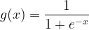
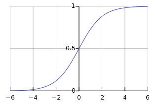
Next step in the study of machine learning is typically the logistic regression. Logistic regression, although termed ‘regression’ is not a regression method. It is essentially a binary classification method that identifies and classifies into two and only two classes. Logistic regression is based on the use of the logistic function, the well known.
|
(1) |
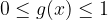
which has a very convenient range of values and a really handy differentiation property,
|
(2) |

|
(3) |
* the logistic function @ -4.6 becomes practically zero (0.01) and @ 4.6 becomes practically one (0.99).
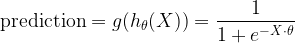
In logistic regression, instead of computing a prediction of an output by simply summing the multiplications of the model (hypothesis) parameters with the data (which is practically what linear regression does), the predictions are the result of a more complex operation as defined by the logistic function,
|
(4) |
where 


![\displaystyle \theta= \left[ \theta_0\quad \theta_1\quad \dots\quad \theta_D \right] ^\intercal](https://s0.wp.com/latex.php?latex=%5Cdisplaystyle+%5Ctheta%3D+%5Cleft%5B+%5Ctheta_0%5Cquad+%5Ctheta_1%5Cquad+%5Cdots%5Cquad+%5Ctheta_D+%5Cright%5D+%5E%5Cintercal&bg=ffffff&fg=000&s=1&c=20201002)
|
(5) |
The predictions resulting from this vectorised operation are all stored in a 

The typical cost function usually used in logistic regression is based on cross entropy computations (which helps in faster convergence in relation to the well known least squares); this cost function is estimated during each learning iteration for the current values of
![\displaystyle J(\theta) = \frac{1}{M} \left[ -y^\intercal \mathrm{log}(h_\theta) - (1-y)^\intercal \mathrm{log}(1-h_\theta) \right]](https://s0.wp.com/latex.php?latex=%5Cdisplaystyle+J%28%5Ctheta%29+%3D+%5Cfrac%7B1%7D%7BM%7D+%5Cleft%5B+-y%5E%5Cintercal+%5Cmathrm%7Blog%7D%28h_%5Ctheta%29+-+%281-y%29%5E%5Cintercal+%5Cmathrm%7Blog%7D%281-h_%5Ctheta%29+%5Cright%5D&bg=ffffff&fg=000&s=1&c=20201002)
|
(6) |
Practically, the above operation may result in computations with infinity, so one might implement it in a slightly tricky way,
% estimate the number of samples in the data
samples = size(X,1);
% estimate the predictions of the inputs according to the current theta parameters
h = 1./(1+exp(-X*theta));
% check where the training class is 0
zero_y = find(y==0);
% check where the training class is 1
one_y = find(y==1);
% evaluate the main cost function formula
cst = - (sum(log(1-h(zero_y))) + sum(log(h(one_y)))) / samples;
During the main algorithm in logistic regression, each iteration updates the
|
(6) |
which updates all the values of 

% computation of the prediction
h = 1./(1+exp(-X*theta));
% simultaneous update of theta
theta = theta - (alpha/M) * (X' * ( h - y));
Apparently this piece of code is what happens within each learning iteration. After this code (and still inside the loop of the training iterations) some kind of convergence criterion should be included, like an estimation of the change in the cost function or the change in the parameters
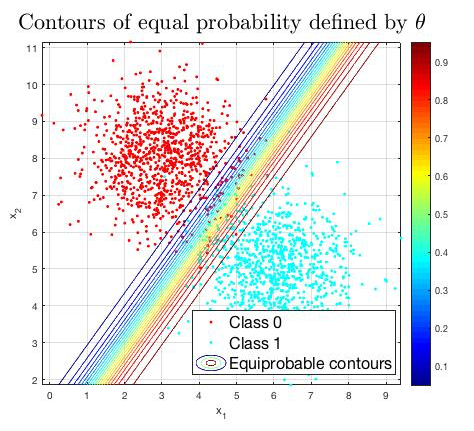
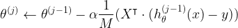
Let’s see what happens when this algorithm is applied in a typical binary classification problem. Suppose there are two sets of 1000 2D training samples following gaussian distributions (for simplicity and illustration). Taken that there are only first-order data (linear terms only, 
After this training process, the prediction formula 

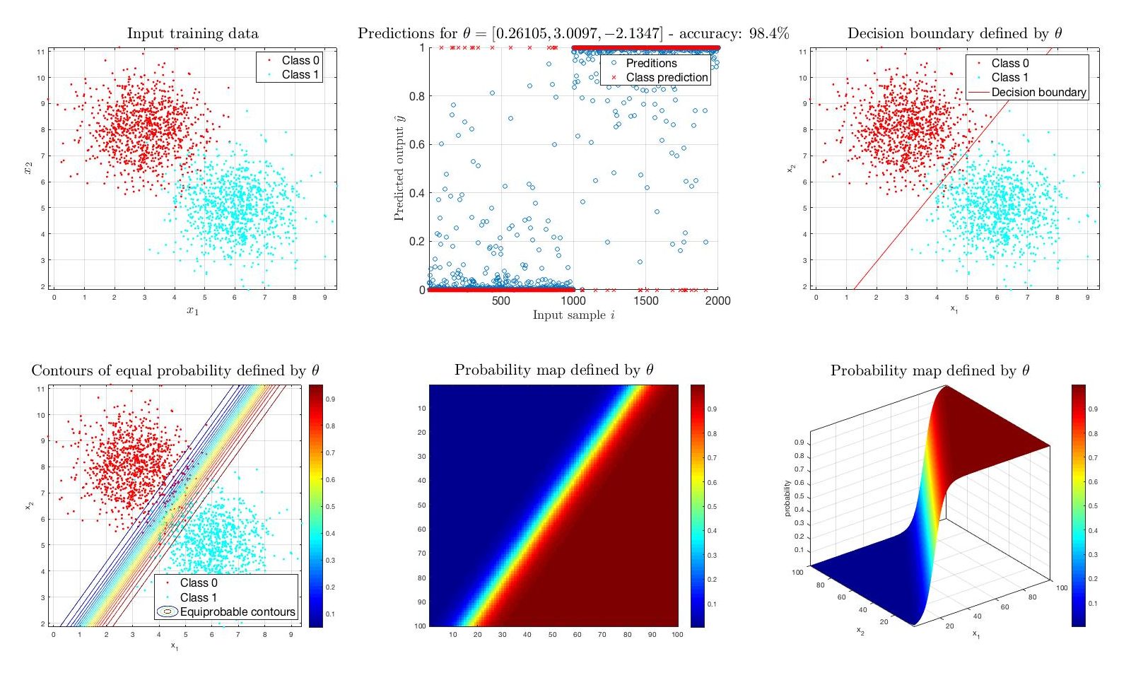
Everything seems perfectly fine in cases in which binary classification is the proper task. If there are more than two classes (i.e. it is a multi-class classification problem) then logistic regression needs an upgrade. This upgrade is not any sophisticated algorithmic update but rather a naive approach towards a typical multiple classifier system, in which many binary classifiers are being applied to recognise each class versus all others (one-vs-all scheme). One has to keep in mind that one logistic regression classifier is enough for two classes but three are needed for three classes and so on.
The following figure presents a simple example of a classification training for a 3-class problem, again using gaussian data for better illustration and only linear terms for classification.
The situation gets significantly more complicated for cases of, say, four (4) classes. Let’s examine a case of 4 classes, in which only linear terms have been used as features for the classification. In the figure that follows it is evident that the decision boundaries are not at all optimum for the data and the training accuracy drops significantly, as there is no way to linearly separate each of the classes.
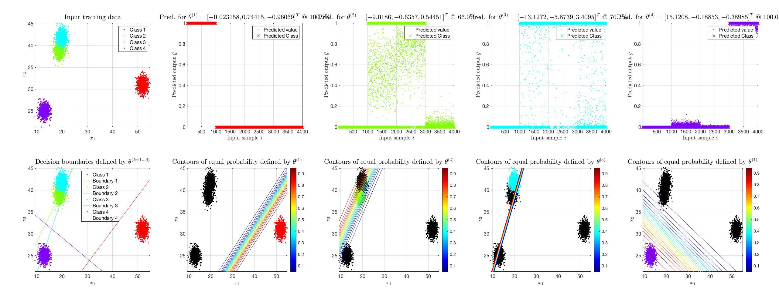
The way to get through with situations like this is to use higher order features for the classification, say second order features like 
![[ x_1,\, x_2,\, x_1^2,\, x_2^2,\, x_1\cdot x_2 ]](https://s0.wp.com/latex.php?latex=%5B+x_1%2C%5C%2C+x_2%2C%5C%2C+x_1%5E2%2C%5C%2C+x_2%5E2%2C%5C%2C+x_1%5Ccdot+x_2+%5D&bg=ffffff&fg=000&s=0&c=20201002)
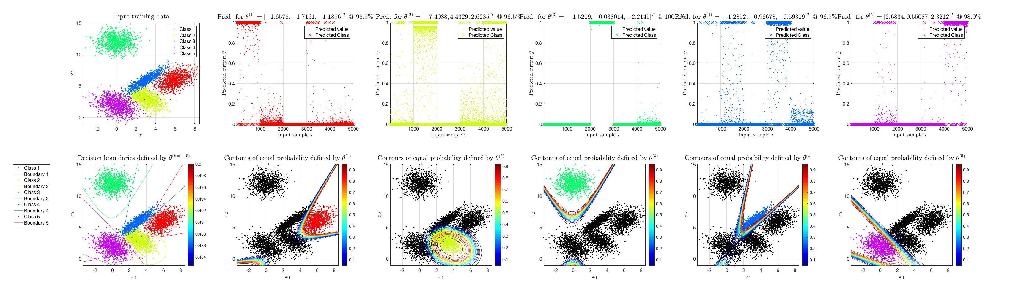
* in this figure only the first 3 of the 5 θ values are shown due to space limitations.
Apparently, this is a completely different picture. Although nothing has changed in the algorithm and the code given above, now the classes are successfully separated by curves. Of course, in this case, as the dimensionality of the training data increases so does the parameter space and the
In multi-class classification applications using logistic regression, similar to binary classification, the response of each of the classifiers (the prediction) represents the probability of each unknown input to be in the ‘Class 1’ of each classifier.
