Of the most basic forms of a machine learning system based on neural networks is the one in which training is accomplished using back error propagation, or simply back-propagation. Back-propagation is a technique, like many others, that targets the minimisation of a cost function during a learning process by following the descending gradient of the function that defines that cost. Similarly to linear or logistic regression (presented in a previous post), it can be seen as a pure cost function minimisation method, in which the definition of the cost and the estimate of the gradient of the cost function are slightly more complex than in the previous cases.
The focus in this post is on a classical network of nodes (or neurons) of a typical logistic (sigmoid) response in the range ![[0,1]](https://s0.wp.com/latex.php?latex=%5B0%2C1%5D&bg=ffffff&fg=000&s=0&c=20201002)
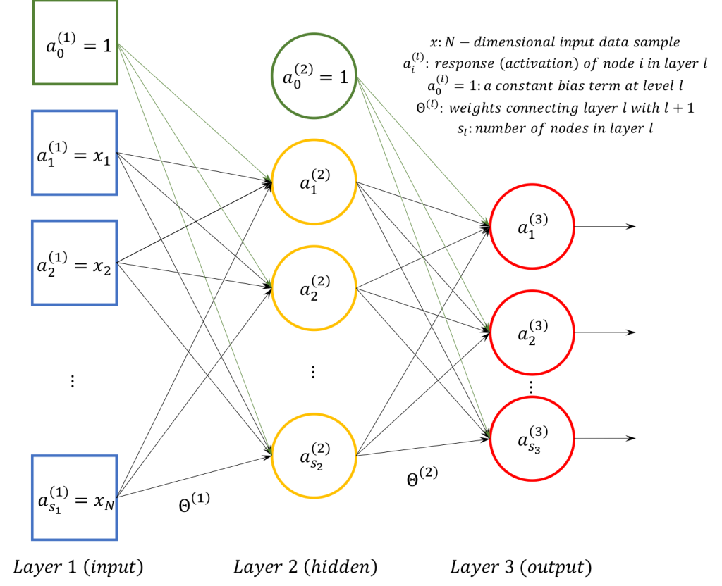
For the supervised training of such a network a number of input examples and the accompanying labels (classes) are required. The training set consists of ![X: [M\times N]](https://s0.wp.com/latex.php?latex=X%3A+%5BM%5Ctimes+N%5D&bg=ffffff&fg=000&s=0&c=20201002)


![y: [M\times 1]](https://s0.wp.com/latex.php?latex=y%3A+%5BM%5Ctimes+1%5D&bg=ffffff&fg=000&s=0&c=20201002)
- Initialisation: initial setting of the weights of the layers’ connections
- Iteration: iterate the following steps until some convergence criteria are met
- Forward propagation: propagation of each input sample all the way through the layers to the output to get the overall hypothesis
- Cost estimation: estimation of the total cost of using the current prediction model (weights) by using the logistic regression cost formula (with or without regularisation)
- Back propagation: propagation of the output error all the way back to obtain a gradient for the model (weights)
- Optimisation: use of an optimisation algorithm to minimise the cost function estimated by the forward propagation using the gradients estimated by the pack-propagation (and derive new weights)
Forward propagation in this particular case has nothing different in essence when compared to logistic regression as described here, so its implementation does not need any more analysis. Particularly interesting though is the back-propagation part of the method. In a somewhat informal description, back-propagation relies on the estimate of the errors that each of the network nodes produces in order to propose a correction of all the model parameters (the weights). It works from the output all the way back to the input using the following computations:
1. computation of divergence from the correct response at the output
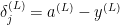

![y^{(L)}= [0 \dots 1 \dots 0]^T](https://s0.wp.com/latex.php?latex=y%5E%7B%28L%29%7D%3D+%5B0+%5Cdots+1+%5Cdots+0%5D%5ET&bg=ffffff&fg=000&s=0&c=20201002)

2. computation of all other divergences

where 

![\dot{g}(z)=g(z)[1-g(z)]](https://s0.wp.com/latex.php?latex=%5Cdot%7Bg%7D%28z%29%3Dg%28z%29%5B1-g%28z%29%5D&bg=ffffff&fg=000&s=0&c=20201002)


3. accumulation of scaled divergences
for layer 


4. computation of the gradient of the cost function


Finally, it should be noted that the cost function taking into account regularisation is formulated as,
![J( \Theta ) = - \frac{1}{M} \left[ \sum\limits_i y \mathrm{log}(h) - (1-y) \mathrm{log}(1-h) \right] + \frac{\lambda}{2M} \sum\limits_j \Theta^2](https://s0.wp.com/latex.php?latex=+J%28+%5CTheta+%29+%3D+-+%5Cfrac%7B1%7D%7BM%7D+%5Cleft%5B+%5Csum%5Climits_i+y+%5Cmathrm%7Blog%7D%28h%29+-+%281-y%29+%5Cmathrm%7Blog%7D%281-h%29+%5Cright%5D+%2B+%5Cfrac%7B%5Clambda%7D%7B2M%7D+%5Csum%5Climits_j+%5CTheta%5E2&bg=ffffff&fg=000&s=0&c=20201002)
Apparently this is an iterative method with multiple inner iterations for the various computations. It turns out that MATLAB/Octave provides a very convenient way of implementing such algorithms using matrix operations that significantly speed up the processes. Supposing that all network matrices (the weights 


% general variables required
% X is the MxN set of training examples
% y is the Mx1 vector of labels for each of the training examples
% m is the number of data samples
% num_layers is the number of layers in the network counting also the input and output
% num_labels is the number of labels / output notes
% lambda is the regularisation parameter

%******************************** FORWARD PROPAGATION
a{1} = X;
for i=2:num_layers
	z{i} = [ones(size(a{i-1},1),1) a{i-1}]*Theta{i-1}';
	a{i} = 1.0 ./ (1-exp(-z{I}));
end

%******************************** COST ESTIMATION
J = 0;
for k=1:num_labels
	% create the output response for each label in the training set
	yy = (y==k);
	% compute cost without regularisation
	J = J - (yy'*log(a{end}(:,k))+(1-yy)'*log(1-a{end}(:,k)))/m;
end
% add up the regularization quantity to the cost
regularisationSum = 0;
for i=1:num_layers-1
	regularisationSum = regularisationSum + sum(sum(Theta{i}(:,2:end).^2));
end
J = J + ((lambda/(2*m)) * regularisationSum);

%******************************** BACK PROPAGATION
% initialise the gradients
for i=2:num_layers
	Theta_grad{i-1} = zeros(size(Theta{i-1}));
end
% create the ground truth output matrix
yy= zeros(m,num_labels);
for i=1:m
	yy(i,y(i)) = 1;
end
% run the back error propagation in matrix form
d{num_layers} = a{num_layers}-yy;
for i=num_layers-1:-1:1
	g_grad = (1.0 ./ (1-exp(-z{I}))) .* (1 - (1.0 ./ (1-exp(-z{I}))));
	d{i} = (d{i+1}*Theta{i}) .* [ones(m,1) g_grad];
	d{i} = d{i}(:,2:end);
	D{i} = d{i+1}'*[ones(size(a{i},1),1) a{i}] / m;
	grad{i} = D{i} + [zeros(size(Theta{i},1),1) (lambda/m) * Theta{i}(:,2:end)];
end
If this piece of code is written as a function (named costFcn()), it is a typical cost function routine, in complete analogy with cost functions in linear or logistic regression. The output of this function should be the cost variable J and the gradient variable grad. Then this function can be passed to an optimisation function in MATLAB/Octave, like fminunc, to obtain a trained network, as follows:
% definition of the lambda regularisation parameter
lambda = .1;
% definition of the number of optimisation iterations needed
iters = 100;
% definition of the network structure (which is passed to the cost function for easy computations)
% in this example the network has N, 25 and 10 nodes in the 3 layers
network = [size(X,2) 25 10];
% definition of the optimisation settings
options = optimset('GradObj', 'on', 'MaxIter', iters, 'Algorithm', 'trust-region');
% train the neural network using the fmincg function (fast alternative to fminunc)
% that can be found @ https://www.mathworks.com/matlabcentral/fileexchange/42770-logistic-regression-with-regularization-used-to-classify-hand-written-digits?focused=3791937&tab=function
Theta = fmincg(@(t)(costFcn([ones(m,1) X], y, t, lambda, 'nn', network)), randomWeights(network), options);
The referenced function randomWeights() is just an auxiliary function to randomly initialise the weights of the network to break any possible symmetry that would stop the learning process in the nodes.
It is noted that many implementations also suggest unrolling the theta matrices into vectors for easy computations. In addition, the above code can be further optimised for performance but it is posted this way for a clearer understanding of the algorithm.
Evaluation of the training process is easy:
% execute a forward propagation to get the predictions for the data X
% the function forwardPropagate is a function that includes the code
% provided in the definition of the cost function above
prediction = forwardPropagate( Theta, X );
% find the network response for the data X
[~, pred] = max(prediction{end}, [], 2);
% report the training accuracy
fprintf('Training Accuracy: %.2f\n', mean(double(pred == y)) * 100);
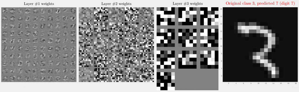
Testing this implementation on a typical application on MNIST data (set of 20×20 graylevel images of handwritten digits) using a network that includes two (2) hidden layers (100 nodes, 25 nodes) on a task to learn to recognise the basic digits 0,1,2,…,9 (10 labels), thus network = [400, 100, 25, 10], lambda set at .1 and 100 optimisation iterations, yields a final cost of around 0.12 and a training accuracy of around 99.4% (it is noted that every test yields slightly different results due to the random initialisation). The following figure presents a visualisation of the weights between each layer, along with a misclassification example.