
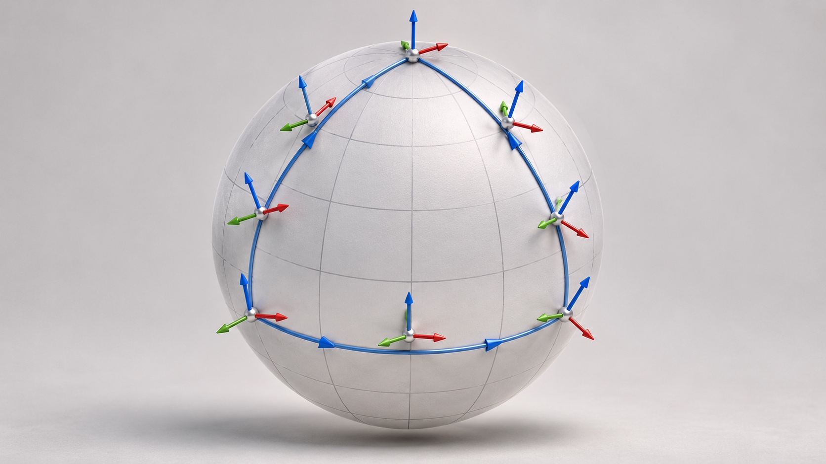
A representation can look similar at two endpoints while behaving differently along the path between them. To see why, imagine carrying a direction through a sequence of local coordinate changes. Returning to the starting location does not, by itself, tell us whether the carried direction has returned to its original orientation.
Holonomy gives a language for that accumulated transformation. Before estimating it in a neural network, it is useful to understand the matrix calculation on a small example.
Research context
Gauge-invariant representation holonomy, by Vasileios Sevetlidis and George Pavlidis, was first posted on 29 January 2026 and appears in ICLR 2026 proceedings. The estimator uses whitening, shared local subspaces and rotation-only Procrustes alignment, then composes local transports. Its invariance claims have conditions on the representation and estimation procedure. The example below uses prescribed rotations; it does not estimate the paper’s statistic from learned features or establish a model’s robustness.
Compose the local operations in order
If R₀ moves a column vector across the first edge and R₁ moves it across the second, the result is R₁R₀v. The rightmost matrix acts first. For a closed sequence of L edges, write:
A natural question is whether H is the identity. Returning to the same input location and returning to the same transported orientation are different requirements. The calculation also depends on using a consistent definition of transport along every edge.
Why three dimensions make a good toy example
Rotations around different axes generally do not commute. Rotate around one axis, then another, then undo the first rotation and undo the second. Each individual operation has an inverse, but this particular sequence need not cancel because the inverses are not adjacent to their original operations.
The accompanying code uses a 25-degree rotation around z and a 35-degree rotation around x. It composes the four edge operations by left multiplication. As a control, using rotations around the same axis makes the corresponding loop close to identity at floating-point precision.
H = np.eye(3)
for edge in [A, B, A.T, B.T]:
    H = edge @ H
assert np.allclose(H.T @ H, np.eye(3))
assert np.isclose(np.linalg.det(H), 1.)
Transposes are inverses here because the matrices are orthogonal. That shortcut would be wrong for an arbitrary matrix.
Change the coordinate frame without changing the question
Suppose U is an orthogonal change of basis. The same accumulated operation is represented in the new coordinates by UHUᵀ. Its entries can look different, but a suitable scalar comparison with identity should not depend on that coordinate choice.
For this example we use the normalized Frobenius gap:
For a p-dimensional orthogonal matrix it lies between zero and one. Orthogonal conjugation preserves the Frobenius norm, so h(UHUᵀ) equals h(H). The code verifies this with a separately generated orthogonal basis.
That invariance is a mathematical property of this construction. It does not mean every preprocessing operation is harmless. Removing coordinates, using different neighborhood samples or estimating a poorly conditioned covariance can change the object being measured.
From matrices to representations
In a network, the local transports must be estimated from feature neighborhoods. That introduces practical choices absent from our four prescribed rotations: the neighborhood definition, shared sample indices, centering, whitening, retained subspace dimension and orientation constraint. A poorly identified alignment can produce an apparent accumulated transformation even when it is mostly estimation noise.
A useful evaluation would include repeated neighborhood samples, a controlled linear baseline and a sensitivity check for loop size and discretization. Comparing models also requires a common protocol. Otherwise an apparent geometric difference may come from different preprocessing or numerical conditioning.
What the example actually establishes
The runnable calculation verifies three things: ordered rotations need not cancel, a same-axis control does cancel, and the normalized gap is invariant under an orthogonal change of basis. It supplies intuition and a software sanity check.
It does not prove that a network has intrinsic curvature, that two models with different gaps have different accuracy, or that a model is adversarially robust. Those questions require the estimator, its assumptions and an appropriate empirical study. Keeping those levels separate makes the geometry more useful, because the reader can tell which statement was calculated and which remains a research question.
Complete reproducible example
This standalone example uses fictional data or prescribed mathematical objects; it is not a reproduction of the source paper’s experiments.
"""Prescribed rotation loop; not a neural-feature holonomy estimator."""
import json
import numpy as np

def rz(deg):
    a=np.deg2rad(deg); c,s=np.cos(a),np.sin(a)
    return np.array([[c,-s,0],[s,c,0],[0,0,1.]])
def rx(deg):
    a=np.deg2rad(deg); c,s=np.cos(a),np.sin(a)
    return np.array([[1.,0,0],[0,c,-s],[0,s,c]])
def compose(edges):
    H=np.eye(3)
    for R in edges: H=R@H
    return H
def gap(H): return np.linalg.norm(H-np.eye(len(H)),'fro')/(2*np.sqrt(len(H)))
A,B=rz(25),rx(35)
H=compose([A,B,A.T,B.T])
U,_=np.linalg.qr(np.random.default_rng(9).normal(size=(3,3)))
assert np.allclose(H.T@H,np.eye(3)) and np.isclose(np.linalg.det(H),1)
assert np.isclose(gap(H),gap(U@H@U.T))
C=rz(35); flat=compose([A,C,A.T,C.T])
assert gap(flat)<1e-12
assert np.isclose(gap(H),gap(H.T))
print(json.dumps({"normalized_gap":float(gap(H)),"changed_basis_gap":float(gap(U@H@U.T)),"same_axis_control":float(gap(flat))},indent=2))