A function is a rule that maps each of the elements in a domain to one and only one element in a range. The set of all possible elements in the input is the domain D of a function; the set of all possible elements in the output is the range R of a function.
According to this trivial definition, a function takes a set of elements and applies its rule to map to another set of elements, so that each and every domain element is mapped once and only. There are, of course, cases in which an element in the range is the mapping of multiple elements in the domain (like in a constant function).
Typically, although the domain is not mentioned one should always keep in mind that the domain is the set of elements for which the function may be evaluated. There are cases in which the domain has to be carefully considered, like in fractions (remember division by zero) and in even roots (remember the elements in even roots have to be greater or equal to zero). Take a look,
In some cases, the domain is not restricted by the definition of the function but it might be restricted by the application (i.e. in which set of elements it might “make sense” to apply the function, in real world applications).
It is possible to combine and to construct composite functions in various forms, like,
![\displaystyle f(x) + g(x), \; f(x) \cdot g(x), \; f(g(x)) \; [\text{or } ((f \circ g)(x)]](https://s0.wp.com/latex.php?latex=%5Cdisplaystyle+f%28x%29+%2B+g%28x%29%2C+%5C%3B+f%28x%29+%5Ccdot+g%28x%29%2C+%5C%3B+f%28g%28x%29%29+%5C%3B+%5B%5Ctext%7Bor+%7D+%28%28f+%5Ccirc+g%29%28x%29%5D++&bg=ffffff&fg=000&s=1&c=20201002)
For various obvious (and non-obvious) reasons it s possible to visualize a function by creating graphs. Typically a graph can be considered as a visualization of the set of points created by the rule of a function in a coordinate system created by the domain and range of the function.
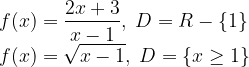
Simple functions of one independent variable, which do not involve powers, etc, like
![\displaystyle f(x) = y = -\frac{3}{2}x+2 \quad [\text{or in general } f(x) = y = ax + b]](https://s0.wp.com/latex.php?latex=%5Cdisplaystyle+f%28x%29+%3D+y+%3D+-%5Cfrac%7B3%7D%7B2%7Dx%2B2+%5Cquad+%5B%5Ctext%7Bor+in+general+%7D+f%28x%29+%3D+y+%3D+ax+%2B+b%5D++&bg=ffffff&fg=000&s=1&c=20201002)
are visualized as straight lines and are called linear. In addition, in these functions it is easy to pinpoint the role of their ingredients a, b as being the slope of the line (the rate of change in the function in respect to the independent variable x) and the y-intercept (where the line crosses y-axis) respectively. It is easy to also pinpoint the x-intercept by equating the function with zero, so putting all together we have
![\displaystyle f(x) = ax + b \\ \text{the slope is } a \left[= \frac{\Delta f(x)}{\Delta x} \right] \\ \text{the y-intercept is } b \left[ = f(x=0) \right] \\ \text{the x-intercept is } f(x) = ax + b = 0 \Rightarrow x_i = -\frac{b}{a}](https://s0.wp.com/latex.php?latex=%5Cdisplaystyle+f%28x%29+%3D+ax+%2B+b+%5C%5C+%5Ctext%7Bthe+slope+is+%7D+a+%5Cleft%5B%3D+%5Cfrac%7B%5CDelta+f%28x%29%7D%7B%5CDelta+x%7D+%5Cright%5D+%5C%5C+%5Ctext%7Bthe+y-intercept+is+%7D+b+%5Cleft%5B+%3D+f%28x%3D0%29+%5Cright%5D+%5C%5C+%5Ctext%7Bthe+x-intercept+is+%7D+f%28x%29+%3D+ax+%2B+b+%3D+0+%5CRightarrow+x_i+%3D+-%5Cfrac%7Bb%7D%7Ba%7D+++&bg=ffffff&fg=000&s=1&c=20201002)
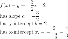
Thus, for example
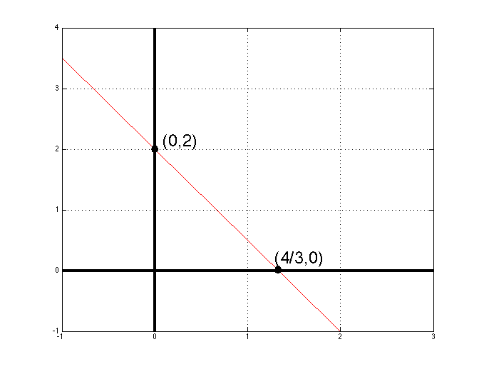
Wanna see how this function’s graph looks like? Take a look,
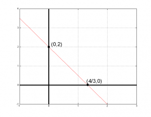
One may easily deduce that

What comes naturally after the study of linear functions is the study of quadratic or second degree functions, that is functions in which the independent variable is raised to the second power.
The standard form of the quadratic functions is

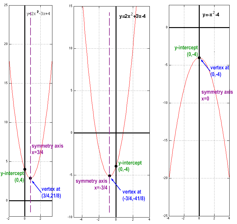
How do quadratic functions look like in graphs? Well, they are parabolas.
If a is positive then the parabola opens up (has a lowest point). If a is negative then the parabola opens down (has a highest point). This lowest or highest point is usually called the vertex. The y-intercept is the constant c,

The x-intercepts can be calculated,

which gives the obvious hint that one quadratic function might have none, one, or at most two x-intercepts!
In addition, the parabola that represents a quadratic function is symmetrically horizontally mirrored around a vertical line that crosses the vertex of the parabola! But where is this vertex? Here it is

*** The computation of the vertex is easy if one considers that this is an extremal of the function and the function is differentiable, thus
![\displaystyle \dot{f} = 2ax+b \xrightarrow[extremals]{for} \dot{f} = 0 \Rightarrow 2ax+b=0 \Rightarrow x = -\frac{b}{2a}](https://s0.wp.com/latex.php?latex=%5Cdisplaystyle+%5Cdot%7Bf%7D+%3D+2ax%2Bb+%5Cxrightarrow%5Bextremals%5D%7Bfor%7D+%5Cdot%7Bf%7D+%3D+0+%5CRightarrow+2ax%2Bb%3D0+%5CRightarrow+x+%3D+-%5Cfrac%7Bb%7D%7B2a%7D++&bg=ffffff&fg=000&s=-1&c=20201002)
…but this is a matter of another post regarding differentiation and derivatives.
How do these functions look like in graphs? Here, take a look
Increasing the power of the independent variable leads to third degree or cubic functions.
The standard form of the cubic functions is

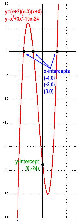
How do cubic functions look like in graphs? Well, they look like recumbent sigmoids S-shapes lying down…
If a is positive then the curve’s right-hand tail opens up, whereas if a is negative then the curve’s right-hand tail opens down. The y-intercept is the constant d,

The x-intercepts can be calculated,
![\displaystyle f(x) = 0 \Rightarrow ax^3 + bx^2 + cx + d = 0 \Rightarrow x_k = -\frac{1}{3a} \left ( b + \zeta^k C + \frac{\Delta_0}{\zeta^k C} \right ), \\ k \in \{0,1,2\}, \; \zeta = -\frac{1}{2} + \frac{1}{2} \sqrt{3} i, \; i \text{ being the complex numbers symbol} \\ \Delta_0 = b^2 -3ac, \; \Delta_1 = 2 b^3 -9abc + 27 a^2 d, \; C = \sqrt[3]{\frac{\Delta_1 \pm \sqrt{\Delta_1^2 -4 \Delta_0^3}}{2}}](https://s0.wp.com/latex.php?latex=%5Cdisplaystyle+f%28x%29+%3D+0+%5CRightarrow+ax%5E3+%2B+bx%5E2+%2B+cx+%2B+d+%3D+0+%5CRightarrow+x_k+%3D+-%5Cfrac%7B1%7D%7B3a%7D+%5Cleft+%28+b+%2B+%5Czeta%5Ek+C+%2B+%5Cfrac%7B%5CDelta_0%7D%7B%5Czeta%5Ek+C%7D+%5Cright+%29%2C+%5C%5C+k+%5Cin+%5C%7B0%2C1%2C2%5C%7D%2C+%5C%3B+%5Czeta+%3D+-%5Cfrac%7B1%7D%7B2%7D+%2B+%5Cfrac%7B1%7D%7B2%7D+%5Csqrt%7B3%7D+i%2C+%5C%3B+i+%5Ctext%7B+being+the+complex+numbers+symbol%7D+%5C%5C+%5CDelta_0+%3D+b%5E2+-3ac%2C+%5C%3B+%5CDelta_1+%3D+2+b%5E3+-9abc+%2B+27+a%5E2+d%2C+%5C%3B+C+%3D+%5Csqrt%5B3%5D%7B%5Cfrac%7B%5CDelta_1+%5Cpm+%5Csqrt%7B%5CDelta_1%5E2+-4+%5CDelta_0%5E3%7D%7D%7B2%7D%7D++&bg=ffffff&fg=000&s=1&c=20201002)
which gives the obvious hint that one cubic function might have none, one, two, or at most three x-intercepts! Since this is extremely tedious, we usually employ factorization (if possible to be easily employed). We would even be really happy if the function was initially given in a factorized form like say,

which otherwise would have been given as,

and it would be really messy…
Following the latter representation we readily know that the curve of this function opens up at the right-hand side (a>0) and that the y-intercept is

Following the factorized representation we readily know the x-intercept points, which are, in this case, three,

And here is how this thing shows up in a graph
Apparently, the third-degree functions are the last of those functions for which to conclude about their appearance in a graph just by looking at their definition (and doing some simple calculations)
The whole concept of such functions generalized to what is called the polynomial functions.
Polynomial functions are the generalized form of n-th degree functions.
The standard form of the n-th degree polynomial functions is

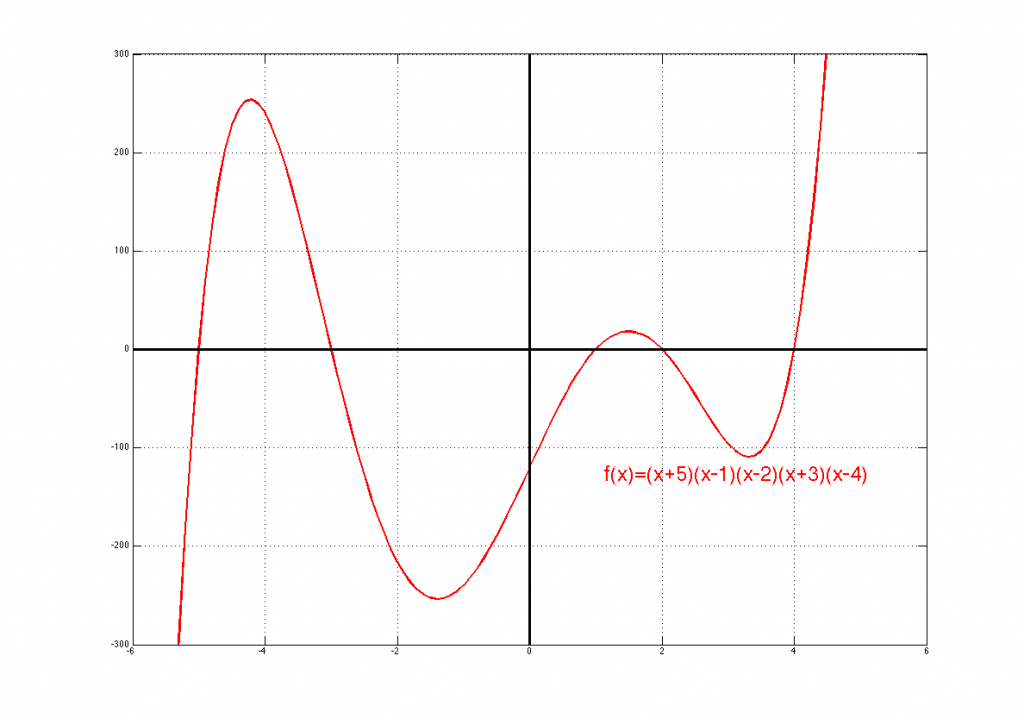
When moving to degrees higher than 4, although there are some clues on how some of them might look there is no formal or informal way to picture them. The things we know is that polynomial functions represent smooth curves without sharp corner edges and breaks.
For example, here is a graph (x-axis is scaled for better illustration) of a fifth degree polynomial function that is defined as