There is a really large number of applications in engineering, in which the identification of critical points of a function is crucial for the analysis and modeling of a process or a system. Generally, one may identify three kinds of critical points, that is (a) maxima, (b) minima and (c) saddle or stationary inflection points.
It is easily understood that in trivial cases (functions that are easy to visualize, like quadratic or cubic curves) a maximum of the function under study occurs in locations where the first derivative of the function equals zero. In a previous post there has been an introduction to such functions and their graphs and it is advised to take a look before continuing.
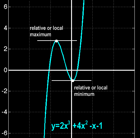
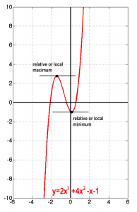
Take for example the cubic function,

is represented by the graph,
The question is how to find those points that at their local neighborhood the seem to be significant by being local maxima or minima. An easy way to tackle this is by remembering that the first derivative of a function at a point can be considered to be the slope of the tangent line at that point. What is different in those interesting points? This tangent seems to be horizontal at those critical points, i.e. it has no slope! Thus, taking the first derivative,
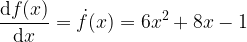
We require that the slope is zero, so,

These are the x positions at which this function exhibits critical points. What kind of points? Till now we cannot tell. We only found out that there are two interesting points for further study…Let’s proceed with what is known. At those locations,
![\displaystyle [f(x)=2x^3+4x^2-x-1] \rightarrow f(x_{1,2}) = \{2.76, -1.06\}](https://s0.wp.com/latex.php?latex=%5Cdisplaystyle+%5Bf%28x%29%3D2x%5E3%2B4x%5E2-x-1%5D+%5Crightarrow+f%28x_%7B1%2C2%7D%29+%3D+%5C%7B2.76%2C+-1.06%5C%7D&bg=ffffff&fg=000&s=1&c=20201002)
That is we have pinpointed the two critical points,

Since we know the graph of the function it is now easy to form an opinion regarding those points: the first is a relative or local maximum and the second a relative or local minimum. Ok this was an easy case.
How about checking the following, again, cubic function,
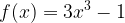
The first derivative of this function is

which, obviously, becomes zero only in the trivial point x=0. This seems at first to be at least problematic: this is a cubic function and one would expect to locate two critical points (since cubic function are supposed to be of a particular shape in their graph). Then, let’s take a look at the graph of this function,
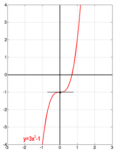
It is easy to see in the graph that the identified critical point cannot be a local maximum of minimum! The function just changes its attitude to the left or to the right of this point. This is what is called a saddle points, or a stationary inflection.
By considering the three cases of critical points already identified, we may state a trivial test to identify critical points in functions as follows
In case of a differentiable function with a critical point at a known location, then,
► If the values of the function to the left and to the right of the critical point are both lower than that of the value at the critical point, then the critical point is a local or relative maximum.
► If the values of the function to the left and to the right of the critical point are both higher than that of the value at the critical point, then the critical point is a local or relative minimum.
► If neither of the above hold then the critical point is a stationary inflection or a saddle point.
This method is very easy to use but requires that there is a knowledge of the graph of the function under study in order to be trivial to identify and classify the critical points. A more general approach is what is called the first derivative test, which is as follows
In case of a differentiable function with a critical point at a known location, then,
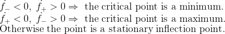
► if the derivative is negative on the left of the critical point and positive on the right, then the critical point is a relative or local minimum.
► if the derivative is positive on the left of the critical point and negative on the right, then the critical point is a relative or local maximum.
► if derivative has same sign on both sides of the critical point then the critical point is a stationary inflection or a saddle point.
In simplified math form,
Let’s reconsider the previous examples, say
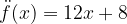
with first derivative
and the obvious single critical point at (0,-1).
On the left of this critical point, say at position x=-1,
On the right, say at position x=1,
So the curve seems to be increasing both on the left and on the right of the critical point so according to the first derivative test this critical point is a stationary inflection (or a saddle) point.


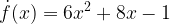
Let us know check the other example, in which,
with first derivative
and two critical points at {(-1.45,2.76),(0.12,-1.06)}. Apparently, we need to consider both critical points, one by one.
On the left of the first critical point (-1.45,2.76), say at position x=-2,
On the critical point, of course the curve levels off.
On the right of the first critical point (-1.45,2.76), and of course on the left of the second point (0.12,-1.06), say at position x=0,
So the first critical point is a local (or relative) maximum.
Moving on to the second critical point, on that point the curve again levels off after decreasing.
Finally on the right of the second critical point (0.12,-1.06), say at position x=1,
So the second critical point is a local (or relative) minimum.


Another elegant way of checking and classifying critical points is based on the usage of the second derivative of the functions under study. The second derivative is the derivative of the first derivative and describes the rate of change of the slope of the tangent on each of the points of the original function. In addition, there is a very helpful mathematical theorem which states that
If the second derivative of a function is positive over an interval then the function is concave up (opens up) over this interval. Equivalently, if the second derivative of a function is negative over that interval then the function is concave down (opens down) over that interval.
This theorem and the definition of the second derivative give rise to the second derivative test for the classification of critical points, which is as follows,
In case of a twice differentiable function with a critical point at a known location, then,
► if the second derivative at the critical point is negative then the function is concave down and the critical point is a relative or local maximum.
► if the second derivative at the critical point is positive then the function is concave up and the critical point is a relative or local minimum.
► if the second derivative at the critical point is null (zero) then the second derivative test fails!
In simplified math form,

Let’s check it through the previously presented examples, starting with the simpler case,
with first derivative
and the obvious single critical point at (0,-1).
The second derivative is
According to the definition of the second derivative test, this critical point cannot be classified with this test!

Let us know check the other example, in which,
with first derivative
and two critical points at {(-1.45,2.76),(0.12,-1.06)}.
The second derivative of this function is
Which leads to the following evaluations of the second derivative in both the critical points,
Clean and easy like this…