Clustering is an important category of machine learning methods and a main form of unsupervised learning. Clustering is essentially distinctive and substantially different from the other dominant form of machine learning, classification, in that it does not rely on training (supervised learning). In principle, clustering represents any method that tries to identify and distinguish groups in data without any prior knowledge of underlying relations and correlations. Usually, clustering methods make use of some distance metric (or measure) to group data based on the similarity that is implied by that metric; typically these methods are iterative, improving the prediction of the clusters in each iteration.
One of the most widely used clustering methods is k-means. K-means is a very simple method which essentially
- begins by randomly initialising the centroids
of the pre-supposed
clusters in the data as
- assigns the data to the clusters that are represented by the centroids based on a similarity metric (or measure) like the L-2 norm (Euclidean distance)
- updates the centroids to reflect the average of the clustered data
- checks for a convergence criterion (ex. no further update in the centroids) and either ends or returns to step 2
Intrinsically, k-means relates to the minimisation of the cost function that is defined by the similarity metric (or measure) used to group data samples in step 2. This cost function can be expressed as
As long as this cost function is differentiable (although there can be nondifferentiable optimisation), in the context of gradient descent optimisation, k-means can be viewed as the process of minimising this cost function
Solving this minimisation problem turns out to give a simple expression
that is, the negative mean distance of the clustered data from the corresponding cluster centroid, where is the number of samples in cluster
; essentially, this expresses a correction that is needed for each centroid according to the currently clustered data.
Since there is a cost function and its gradient, k-means has been ‘transformed’ into a gradient minimisation problem, solved just like linear or logistic regression. This can be easily translated into a Matlab/Octave function as follows:
function [J,grad] = costFcnKmeans( X, W )
	% understand the data and dimensions
	K = size(W,1);
	m = size(X,1);
	n = size(X,2);
	% take the euclidean norm as a distance factor
	for k=1:K
		d(:,k) = sum((X-W(k,:)).^2,2);
	end
	% get the min distances and associated classes
	[d, c] = min( d,[],2 );
	% estimate the cost of having the current centroids
	J = (d'*d) / (2*m);
	% estimate the gradient of the cost
	grad = zeros(K,n);
	for k=1:K
		grad(k,:) = -sum( X(c==k,:)-W(k,:)) / m;
	end
*** It should be emphasised that the correct formula for the gradient should be:
	denominator = size(X(c==k,:),1);
	grad(k,:) = -sum( X(c==k,:)-W(k,:)) / denominator;
but this needs attention, because in cases in which there are no samples assigned to cluster then
, and the
; simply dividing by the total number of samples guarantees that this never happens and does not actually change the result, although it is expected to change the number of iterations in the optimisation and the first-order optimality estimated. Another solution would be to add a couple more lines of code to address division by zero, like,
denominator = size( X(c==k,:),1);
if denominator ~= 0
	grad(k,:) = -sum( X(c==k,:)-W(k,:)) / denominator;
end
Additionally, one could also include an else in that if (right before the end), to address the case of the denominator actually being zero,
else
	grad(k,:) = -W(k,:);
but this does not make a difference in the result, also.
Using this cost function in optimisation in Matlab/Octave is typically implemented using the fminunc. Here is an example code on how to run a k-means clustering as a cost function minimisation:
% initialise centroids using random samples from the data
% X is the data matrix MxN (M samples of N dimensions)
% clusters is the pre-selected number of clusters (scalar)
% initial_w and w are the centroids matrices KxN (K clusters of N dimensions)
initial_w = X(randperm(M,clusters),:);
% Optimize centroids
options = optimset('GradObj', 'on', 'MaxIter', 100, 'Algorithm', 'trust-region','Display','iter');
w = fminunc(@(t)(costFcnKmeans(X, t)), initial_w, options);
% apply the clustering according to the centroids and get the L-2 distance
for k=1:clusters
	d(:,k) = sum((X-w(k,:)).^2,2);
end
% get the data classes in c from the L-2 distance: c is a Mx1 vector of class labels for the X data
[d,c] = min(d,[],2);
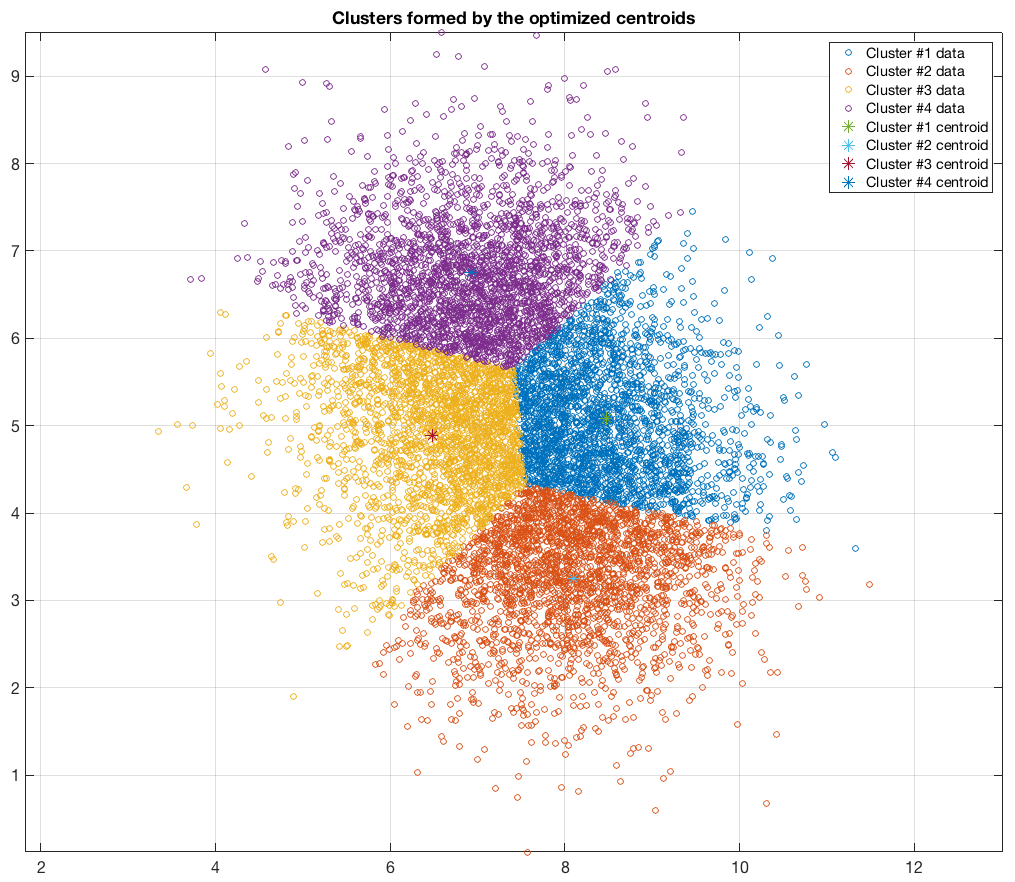
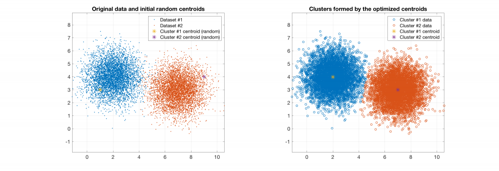
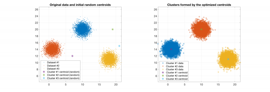
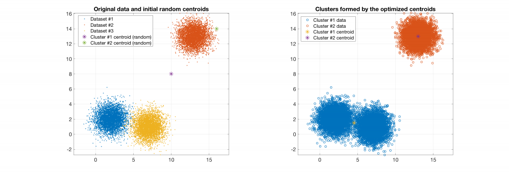
The following figures present some interesting and representative examples of the application of this approach. In these figures, on the left is the original dataset purposely created as a multi class Gaussian mixture along with the initial centroid, whereas on the right is the result of k-means clustering as cost function minimisation based on the L-2 norm using gradient descent.
Data belonging to 2 clusters, 2 clusters requested:

Data belonging to 3 clusters, 3 clusters requested:

Data belonging to 3 clusters, 2 clusters requested:

Data belonging to 2 clusters, 3 clusters requested:

Data belonging to 2 clusters, 4 clusters requested:

Data belonging to 3 clusters, 4 clusters requested, 3 clusters resulted:

Data belonging to 3 clusters, 4 clusters requested, 2 clusters resulted:


